Submission

Introduction

Our project aims to measure the ability of defensive backs at performing different aspects of their defensive duties: deterring targets (either by reputation or through good positioning), closing down receivers, and breaking up passes. We do this by fitting four models, two for predicting the probability that a receiver will be targeted on a given play and two for predicting the probability that a pass will be caught, which we then use to aggregate the contributions of defensive backs over the course of the season.

Modeling Framework

We opted to use XGBoost for all of our models. At a high level, we chose a tree booster for its ability to find complex interactions between predictors, something we anticipated would be necessary for this project. Tree boosting also allows for null values to be present, which helped us divvy up credit in the catch probability models (more on this later). Finally, tree boosting is a relatively simple, easy to tune algorithm that generally performs extremely well, as was the case for us.

Catch Probability

Our catch probability model has two distinct components: The catch probability at throw time – as in, the chance that the pass is caught at the time the quarterback releases the ball – and the catch probability at arrival time – the chance the pass is caught at the time the ball arrives. These probabilities are clearly distinct, since a lot can happen between throw release and throw arrival. First, we will walk through the features that are used in building each model.

For the throw time model (which we will refer to as the “throw” model) and the arrival time model (the “arrival” model), the most important predictors by variable importance were what we expected entering this project: the distance of the receiver to the closest defender, the position of the receiver in the \(y\) direction (i.e. distance from the sideline), the distance of the throw, the position of the football in the \(y\) direction at arrival time (this is mostly catching throws to the sideline and throw aways), the velocity of the throw, the velocity and acceleration of the targeted receiver, and a composite receiver skill metric. For the arrival model, we use many of the same features. However, we do not account for the distance of the defenders to the throw vector – which accounts for the ability to break up a pass mid-flight – because the throw has already arrived.

These two models both perform quite well, and far better than random chance. The throw model accurately predicts \(74\%\) of all passes, with strong precision (\(84\%\)) and recall (\(76\%\)), and an AUC of \(0.81\). As can be expected, our arrival model outperforms the throw model in all measures - accurately predicting \(78\%\) of all passes with a precision of \(88\%\), a recall of \(79\%\), and an AUC of \(.87\). All of these metrics were calculated on a held out data set not used in model training. Below are plots of the calibration of the predictions of each of the models on the same held out set.

 

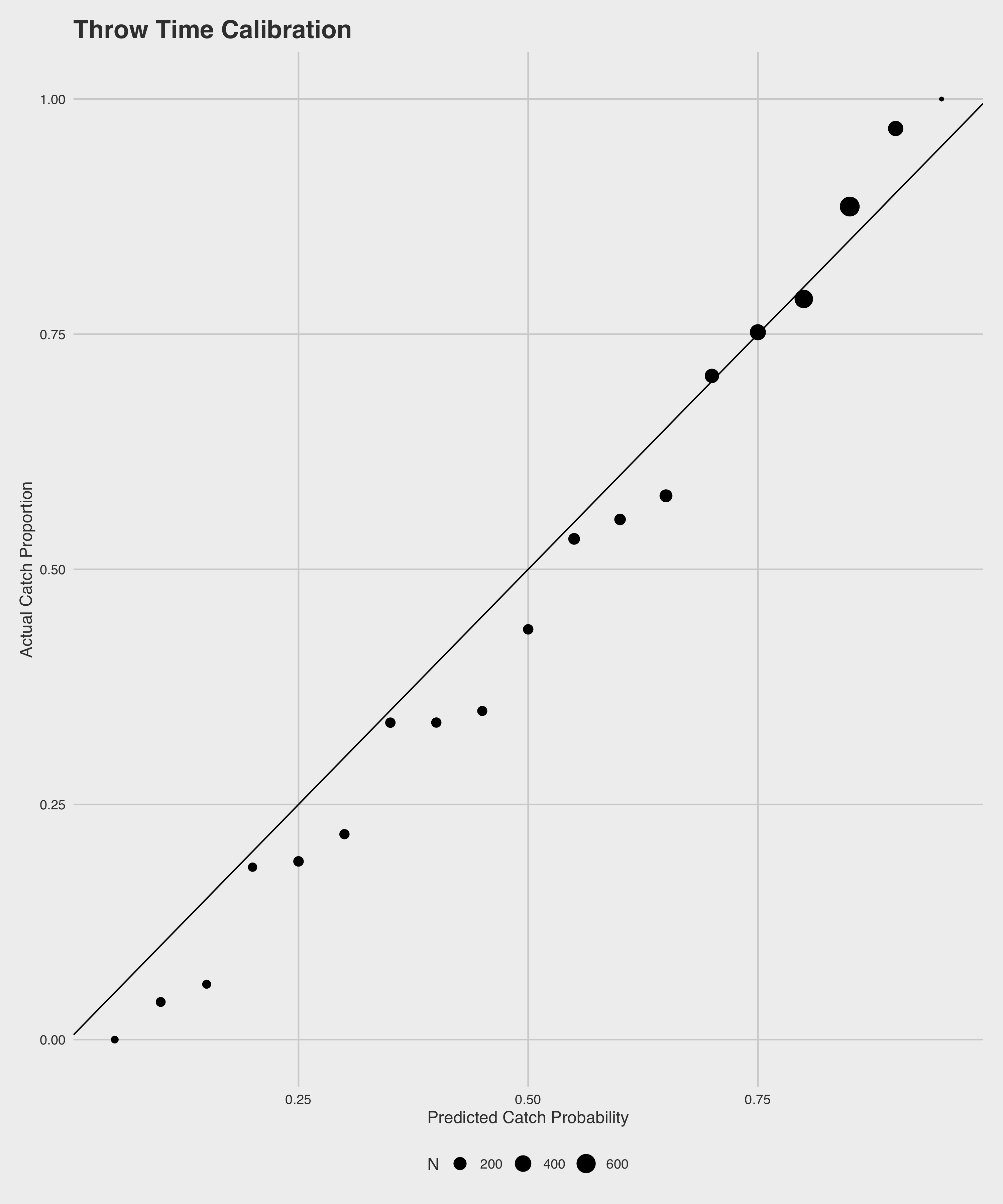
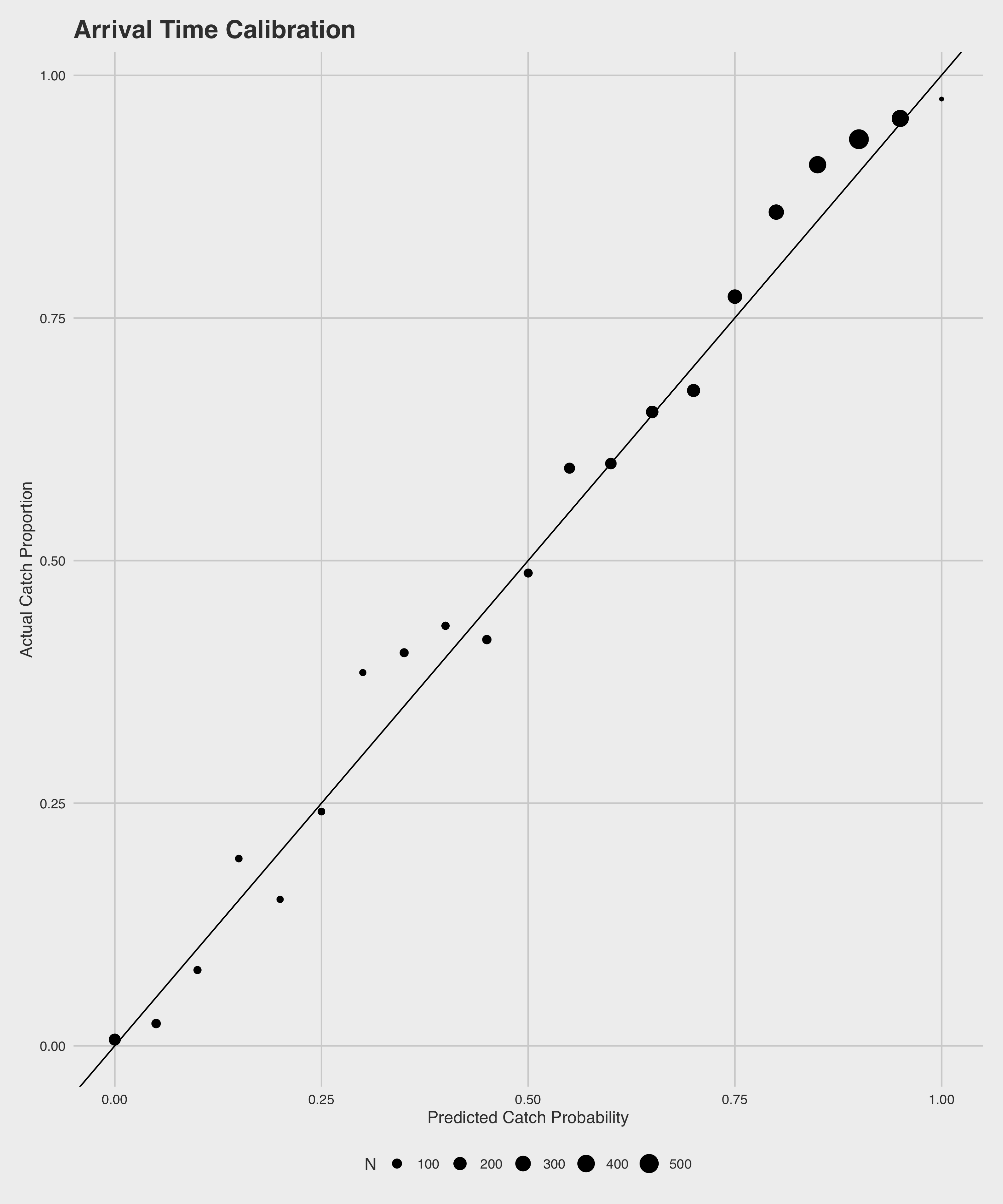
Catch Probability Model Calibration Plots

 

We can do a few particularly interesting things with the predictions from these two models in tandem. Namely, we can use the two to calculate marginal effects of the play of the defensive backs. A simple example is as follows: For a given pass attempt, our throw model estimates that there is a \(80\%\) chance of a catch. By the time that pass arrives, however, our arrival model estimates instead that there is a \(50\%\) chance of a catch. Ultimately, the play results in a drop. In total, our defense can get credit for \(+.8\) drops, but we can break it down into \(+.3\) drops worth from closing on the receiver and \(+.5\) drops from breaking up the play, based on how the individual components differ. In other words, we subtract the probability of a catch at arrival time from the probability at throw time to get the credit for closing down the receiver, and we subtract the true outcome of the play from the probability of a catch at arrival time to get the credit for breaking up the pass.

The main challenge comes not from calculating the overall credit on the play, but from the distribution of credit among the defenders. In the previous example where we have to credit the defense with \(+.8\) drops added, who exactly on the defense do we give that credit to? There are a couple of heuristics that might make sense. One option would be to just split the credit up evenly among the defense, but this would be a bad heuristic because some defenders will have more of an impact on a pass being caught than others, and thus deserve more credit. We might also give all of the credit to the nearest defender, but that would be unfair to players who are within half a yard of the play and are also affecting its outcome but would get no credit under this heuristic. Ultimately, we opted to use the models to engineer the credit each player deserves by seeing how the catch probabilities would change if we magically removed them from the field, which we believe to be a better heuristic than previous ones described. To implement this heuristic, we remove one defender from our data and re-run the predictions to see how big the magnitude of the change in catch probability is. The bigger the magnitude difference, the more credit that player gets. Then, we calculate the credit each defender gets with \(credit_{i} = \frac{min(d_{i}, 0)}{\sum_{i} min(d_{i}, 0)}\) where \(d_{i}\) is the catch probability without that player on the field minus the catch probability with him on the field. In other words, if one player gets \(75\%\) of the credit for a play and the play is worth \(+.8\) drops added, then that player gets \(.8 \cdot .75 = +.6\) drops of credit, and the remaining \(+.2\) drops is divvied up amongst the other defenders in the same fashion.

Target Probability

Our target model is based around comparing the probabilities a receiver is targeted before the play begins and when the ball is thrown with the actual receiver targeted. We can use these probabilities to make estimates of how well the defender is covering (are receivers less likely to be thrown the ball because of the pre-throw work of a defensive back?) and how much respect they get from opposing offenses (do quarterbacks tend to make different decisions at throw time because of the defensive back?).

To determine the probability of a receiver being targeted before the play, we chose to take a naive approach. Each receiver on the field is assigned a “target rate” of \(\frac{targets}{\sqrt{plays}}\), which is then adjusted for the other receivers on the field and used as the only feature for a logit model. The idea of this rate was to construct a statistic which rewarded receivers for showing high target rates over a large sample, but also giving receivers who play more often more credit.

The model for target probability at the time of throw was a tree booster similar to the two catch probability models. This model uses positional data, comparing the receiver position to the QB and the three closest defenders along with a variety of situational factors such as the distance to the first down line, time left, weather conditions, and how open that receiver is relative to others on the play to determine how likely that receiver is to be targeted.

The pre-snap model, which by design only considers the players on the field for the offense, performs relatively well for the lack of information with an AUC of \(.59\) and is well-calibrated on a held-out dataset. The pre-throw model performs much better given the extra information, with \(89\%\) recall, \(94\%\) precision, and \(.94\) AUC. Calibration plots of the models on held-out data are below.

 

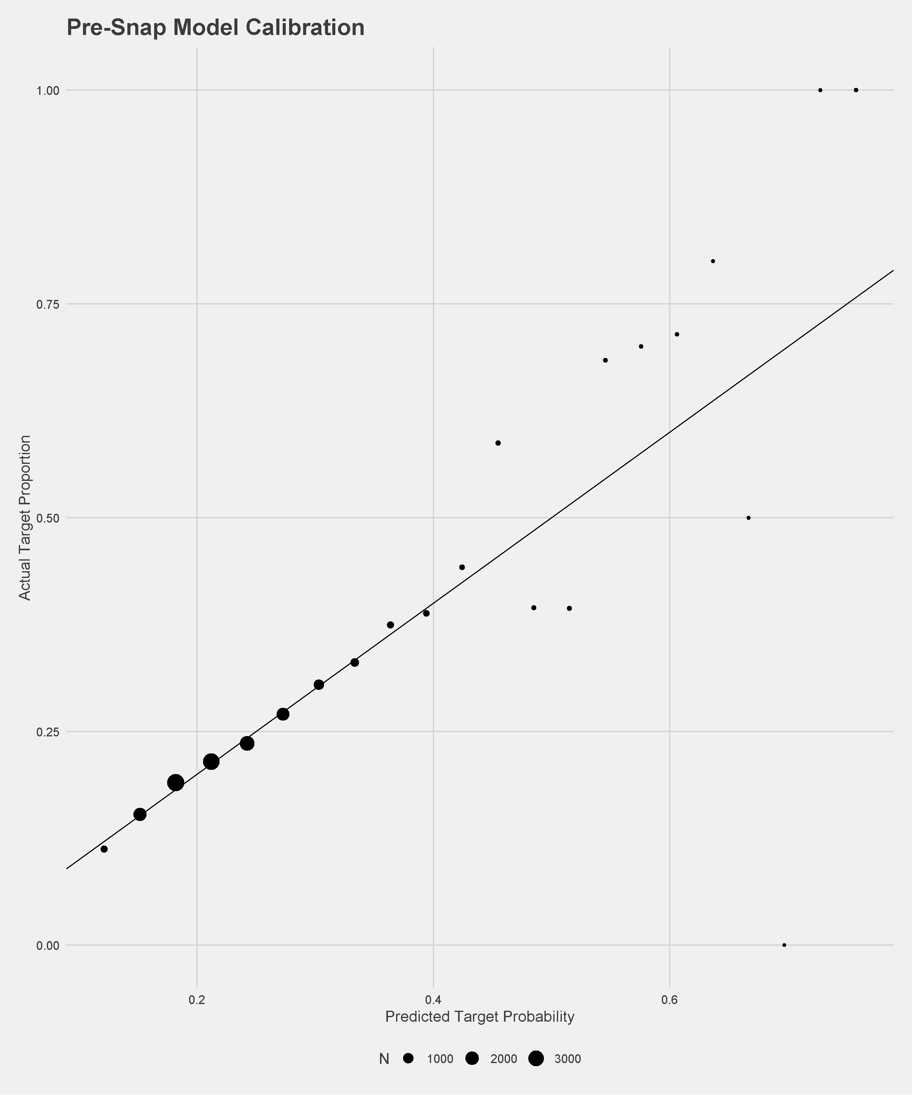
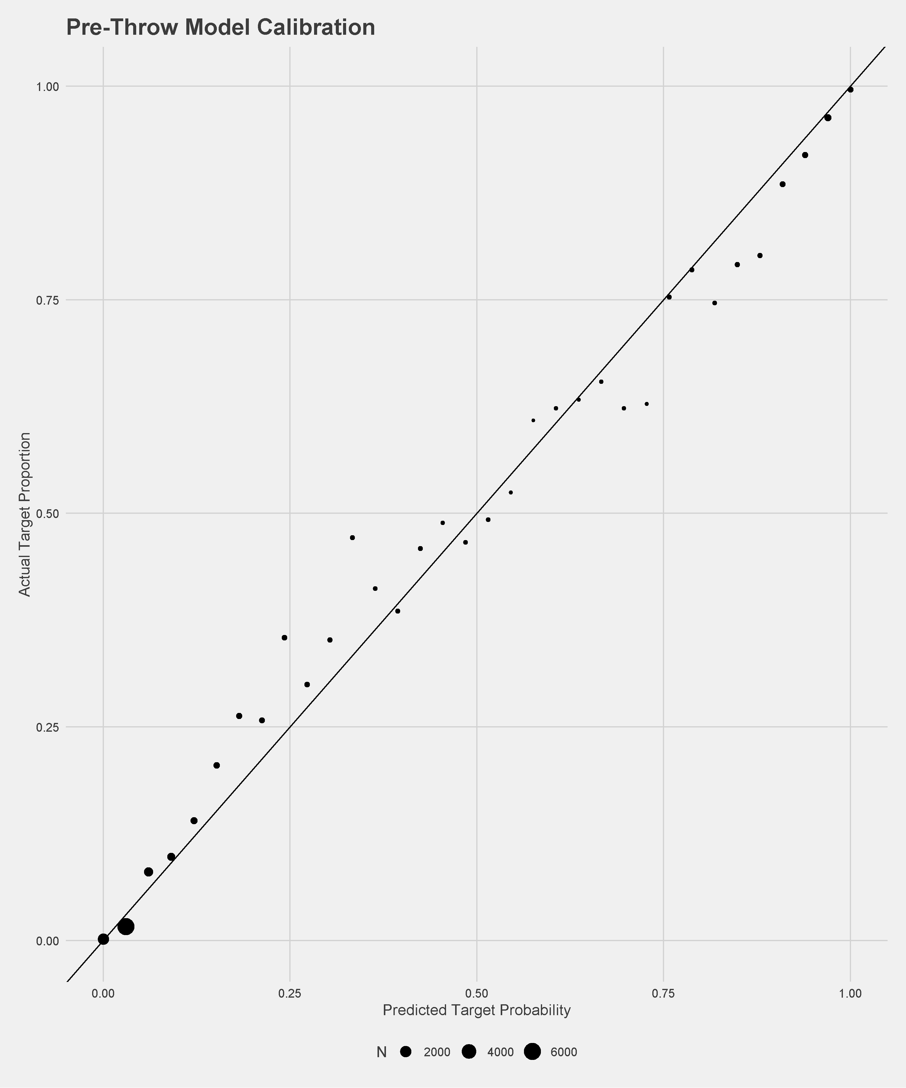
Target Probability Model Calibration Plots

 

We can estimate how a defensive back is impacting the decisions made by the quarterback through two effects. The first, comparing the target probability prior to the play to the target probability at the time of the throw is meant to estimate how well the receiver is covered on the play. For example, consider a receiver with a target probability of \(20\%\) prior to the snap who ends up open enough to get a target probability of \(50\%\) when the ball is thrown. This difference is attributed to the closest defensive back who would be credited with \(-0.3\) coverage targets. If on the same play another receiver had a pre-snap target probability \(30\%\) but a target probability of \(0\%\) at throw time, the closest defensive back would be credited with \(+0.3\) coverage targets. The other effect attempts to measure how the quarterback is deterred from throwing when that particular defensive back is in the area of the receiver by comparing the probability of a target to the actual result. So if a certain receiver has a target probability of \(60\%\) at the time of the throw and isn’t targeted, the closest defender is credited with \(+0.6\) deterrence targets.

Results

Having produced these four models that gave us estimates of the influence of the defensive backs on a given play, we can accumulate the results over an entire season to produce an estimate of individual skill across the dimensions described by the models. As there is not a straightforward way to measure the relative value of these skills, we chose to combine the individual skill percentiles for each defender as a measure of their overall skill. With that as the estimate, these are our top 15 pass defending defensive backs in 2018:

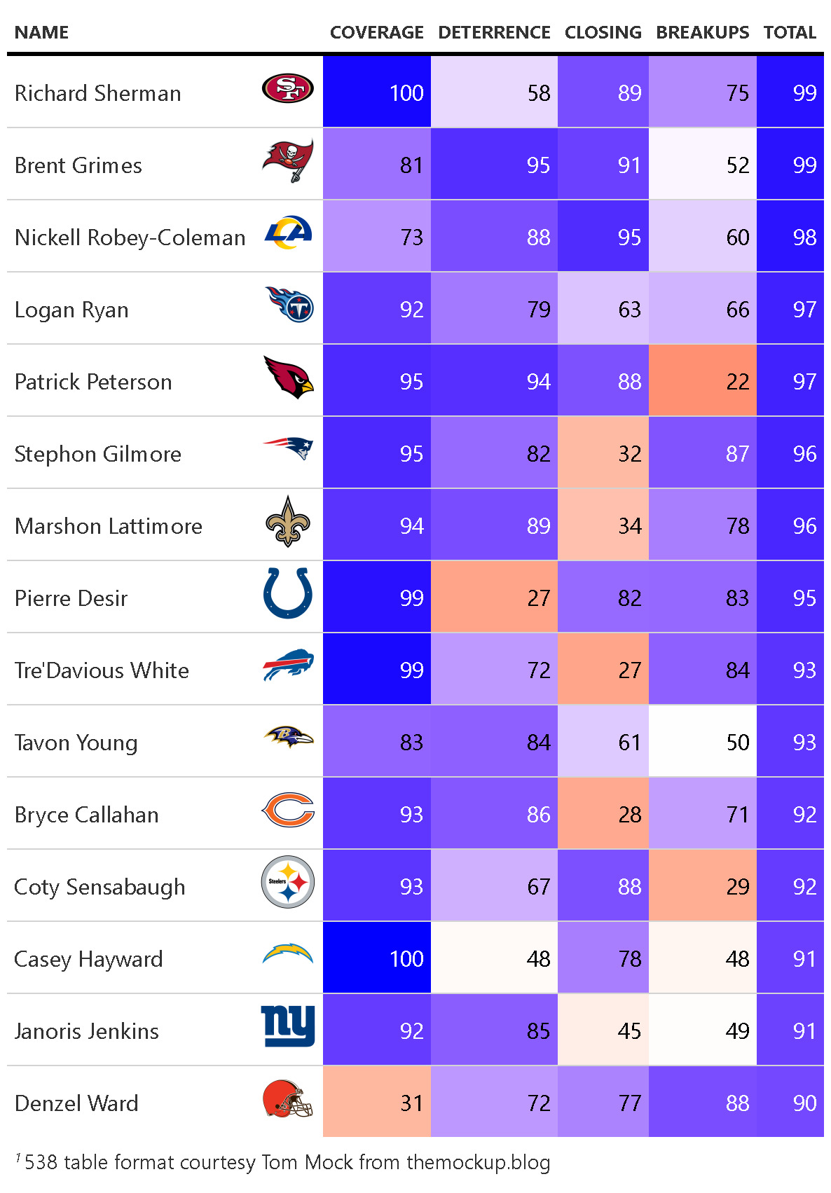
Top 15 Defenders, 2018

A full leaderboard of these can be found on our Shiny app in the Overall Rankings tab. To help display these results and a few other metrics (such as how difficult the defensive assignment was based on pre-snap target probability and actual separation from receiver at throw time) we developed player cards for each qualifying defender. For example, this is our card for #1 defender Richard Sherman:

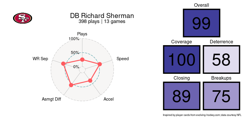
These cards can also be found on our Shiny app under Player Cards.

Further Work

There are a number of things that we didn’t consider or that would be interesting extensions of this project. Two clear ones are interceptions added and fumbles added, as those are hugely impactful football plays that can swing the outcomes of games. We also only considered raw changes in aggregating the player stats (i.e. targets prevented and drops added), but using EPA added instead would certainly be a better metric, since not all drops are created equal. In addition, it is not clear that a drop added is worth the same as a target deterred – an assumption we made – and EPA would help solve this problem too. It would also be interesting to test how similar our metrics are between seasons to confirm that our metrics are measuring the stable skill of a defender.

Appendix

All of our code is hosted in two Github repos: hjmbigdatabowl/bdb2021, which hosts our modeling code, and hjmbigdatabowl/bdb2021-shiny, which hosts the Shiny app.

There is extensive documentation for our code on our pkgdown site.

The Shiny app can be found here, which lets you explore our models, results, and player ratings.